
Sublinear Algorithms for Estimating Single-Linkage Clustering Costs
Finished in 2025
Authors: Pan Peng, Christian Sohler, Yi Xu* (alphabetical order)
Motivation
A single-linkage clustering (SLC) is obtained by iteratively merging the closest pair of clusters, where initially every data point forms its own cluster. Given a weighted graph, construction the SLC hierarchy requires linear time and accessing the whole input, which is not acceptable in big data era. Therefore, our goal is to design informative cost functions to reflect properties of datasets, and then estimate these costs efficiently in sublinear time. This allows us to summarize the clustering structure of data without accessing the whole input.
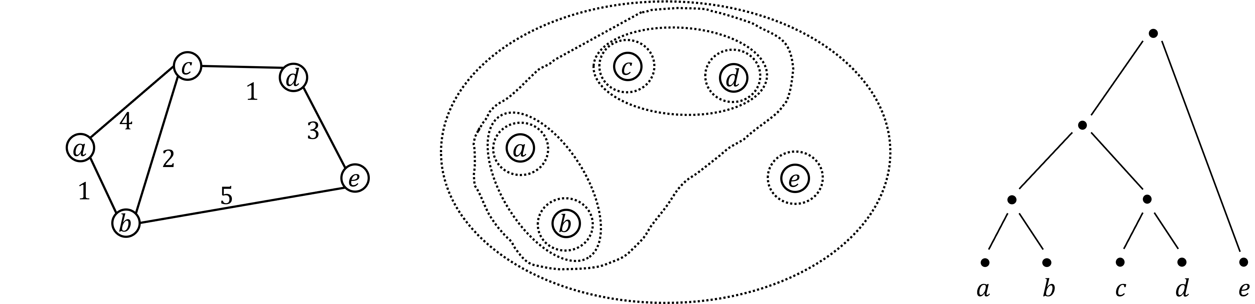
Algorithmically, one can compute a single linkage \(k\)-clustering (a partition into \(k\) clusters) by computing a minimum spanning tree and dropping the \(k-1\) most costly edges.
This clustering minimizes the sum of spanning tree weights of the clusters. This motivates us to define the cost \(\mathrm{cost}_k\) of a single linkage \(k\)-clustering by the weight of the corresponding spanning forest. Besides, if we consider single linkage clustering as computing a hierarchy of clusterings, the total cost of the hierarchy is defined as the sum of the individual clusterings. That is, \(\mathrm{cost}(G) = \sum_{k=1}^n \mathrm{cost}_k\).
The naive method is to compute a minimum spanning tree first, then compute exact values of \(\mathrm{cost}_k\) and \(\mathrm{cost}(G)\), which is linear in time.
Our results
Let \(W\) be the maximum edge weight in the graph, and \(d\) be the average degree. Suppose the input graph is given in ajacency list model, and for any vertex, one can query its neighbor. We give sublinear algorithms to estimate the cost functions, almost matching the lower bound.
| \((1+\varepsilon)\)-estimate of \(\mathrm{cost}(G)\) | Succinct representation of \(\mathrm{cost}_k\) | Lower bound |
|---|---|---|
| \(\tilde{O}(\sqrt{W}/\varepsilon^3 d)\) | \(\tilde{O}(\sqrt{W}/\varepsilon^3 d)\) | \(\Omega(\sqrt{W}/\varepsilon^2 d)\) |
Succinct representation meaning:
For all \(k\), we can recover \(\widehat{\mathrm{cost}_k}\) in a short time, with average \((1+\varepsilon)\) error, which means:
and query time for retrieving each \(k\) is \(O(\log\log W)\).
Techniques
- Reduction: SLC cost estimation reduces to estimating the number of connected components (#CCs) in thresholded subgraphs
- Estimating connected components:
- Use sampling and BFS ([CRT05])
- Our algorithm improves on prior bounds
- Binary search for acceleration:
- Since each #CCs lies in the range \([1,n]\), we partition this range into intervals

- We then map #CCs to the nearest interval endpoints:
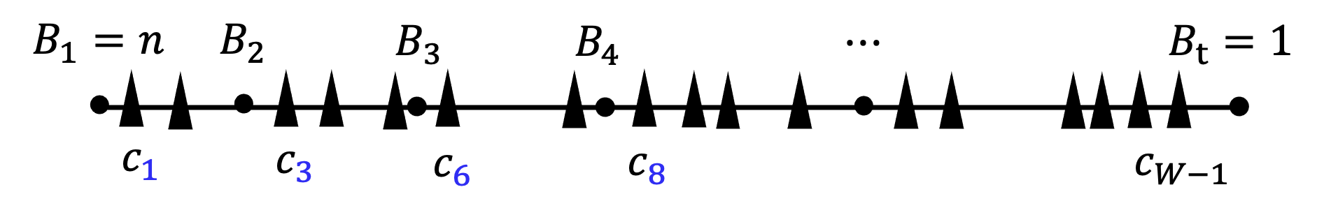
- We choose endpoints wisely, such that the gap of two endpoints are close to the error bound of CC values
Extension: similarity case
We further extend our results to another measurement: every edge weight in graph represents similarity, and in every step of SLC, it merges two most similar clusters.
We note that this measurement is more subtle and challenging to handle, than the distance case.
We obtain a similar result, but the query complexity is linear in \(W\) now (in distance case, it’s linear in \(\sqrt{W}\)).
| \((1+\varepsilon)\)-estimate of \(\mathrm{cost}(G)\) | Succinct representation of \(\mathrm{cost}_k\) | Lower bound |
|---|---|---|
| \(\tilde{O}(W/\varepsilon^3 d)\) | \(\tilde{O}(W/\varepsilon^3 d)\) | \(\Omega(W/\varepsilon^2 d)\) |
Experiments
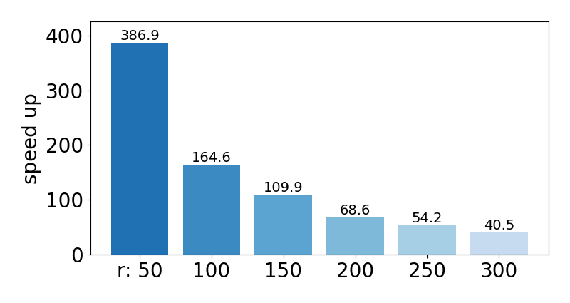
- \(r\): sample size for CC estimation; \(\widehat{\mathrm{cost}_k}\): estimated value for \(\mathrm{cost}_k\).
| Approximation ratio | Speed up for datasets (\(r=100\)) | Speed up for various \(r\) |
|---|---|---|
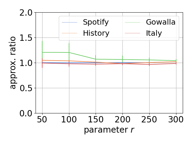 | 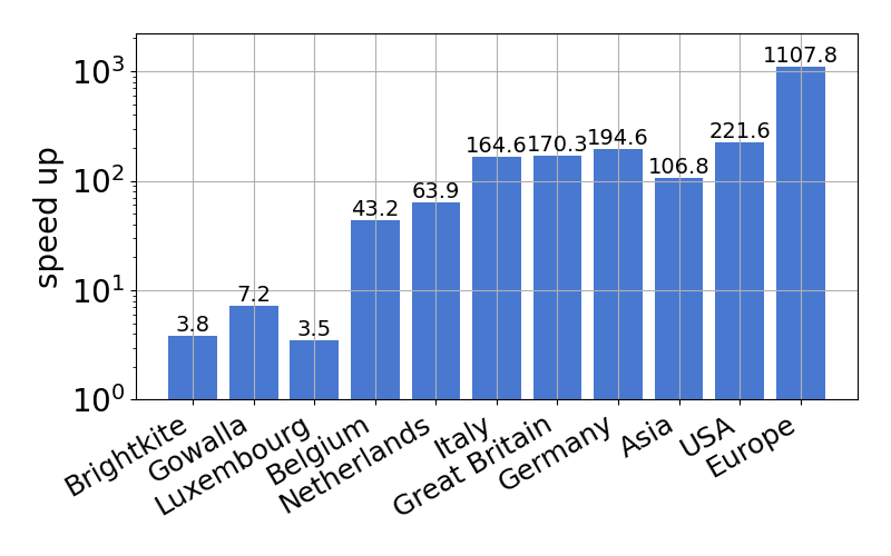 |  |
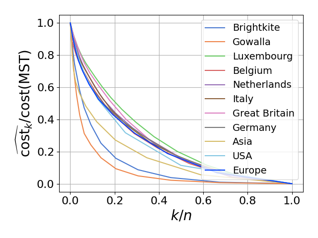
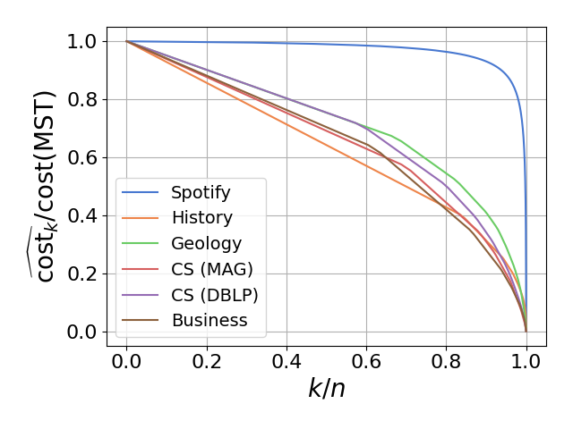
The sequence \(\{\mathrm{cost}_1, \mathrm{cost}_2, \ldots, \mathrm{cost}_n\}\) can be regarded as a profile vector representing the SLC clustering hierarchy. Our experiments demonstrate that these profile vectors can be estimated with high accuracy for each dataset, effectively capturing the intrinsic structural properties of the data.
| Profile in distance case | Profile in similarity case |
|---|---|
 |  |